Part5: Forward Pass

With our dataset prepared and our model's architecture ready, we are at starting point of deep learning. The first part is the forward pass.

In this part, we will implement the entire forward pass from scratch. We will see how input data travls and transforms through our layers. Before we jump into the code, let's look at what the forward pass actually is and examine the components that make it work.

What is the Forward Pass?

The Forward Pass is the process of transforming raw input data into a prediction, and ultimately, calculating a Loss, which is a numerical value representing the difference between the model's prediction and the actual value.

In our network, data flows sequentially from the Input Layer through the Hidden Layer, and finally to the Output Layer.

For each layer in the network, we are esstentiailly calculating the following formula:

$$y = f(xW + b)$$

where:

• x: The input tensor.

• W: The weight matrix.

• b: The bias vector.

• f: The activation function.

The Linear Transformation (xW + b)

Each neural network layer applies a linear transformation to its inputs. The weight matrix W determines how input features are combined, while the bias term b shifts the activation of each neuron. Although the true data-generating process includes a constant term (+20), the bias does not explicitly “store” this value. Instead, it allows the model to learn the correct output offset during training.

The Activation Function (f)

The activation function introduces nonlinearity into the model. Without it, the network could only represent linear functions. By applying nonlinear activations in the hidden layer, the network can construct complex feature representations that allow it to approximate nonlinear relationships such as a cubic function.

The Sequence in our Model

In the network, the "predicted value" is generated by running this formula twice:

Hidden Layer Pass:

$$h = f(xW_{input} + b_{input})$$

Here, x is transformed into different "features" (h) in the hidden layer.

Output Layer Pass:

$$\hat{y} = hW_{output} + b_{output}$$

The features are then compressed back down into a single value: the model’s predicted y.

By the end of the forward pass, the model produces a predicted value. We then compare this prediction to the actual value using a Loss Function to determine how much the model needs to learn during the next phase.

Now that we have a understanding of the forawd pass, it's time to coding. The fist component we will implement is the loss funciton.

Implementing the Loss Function

Let’s start the coding with loss function. There are many loss functions. For regression tasks, the standard choice is Mean Squared Error (MSE). MSE calculates the average of the squares of the difference between the predicted value and the actual target value.

$$MSE = (1/n)*\sum(P_{i} - A_{i})^2$$

Add this method to our SimpleRegressionModel struct implementation:

/// Computes the Mean Squared Error between predictions and targets.
fn compute_loss(&self, logits: Tensor<B, 2>, targets: Tensor<B, 2>) -> Tensor<B, 1> {
    // 1. Calculate the difference (P - A) and square it: (P - A)^2
    let squared_error = logits.sub(targets).powf_scalar(2.0);

    // 2. Calculate the mean of all squared errors in the batch
    squared_error.mean()
}

Tensor Shape Note

• logits: Shape [Batch Size, 1]

• targets: Shape [Batch Size, 1]

• loss: Shape [1] (a scalar value representing the average error of the entire batch).

Implementing the Activation Function

As we discussed, a neural network without an activation function is essentially just a giant linear calculator. To capture the "curves" in our cubic data (\(x^3\)), we need to introduce non-linearity.

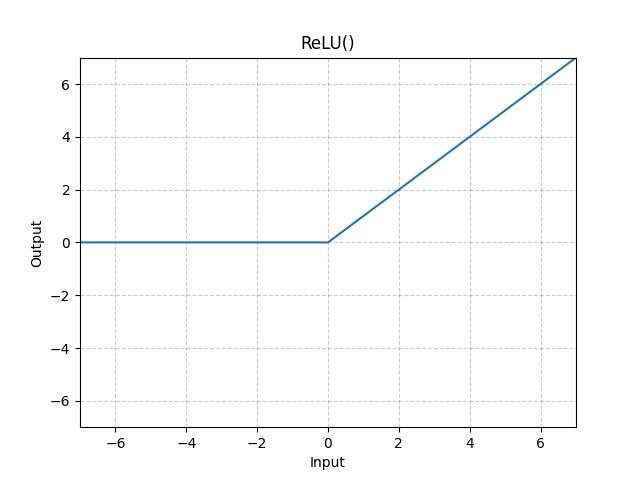
The most popular choice in modern deep learning is the ReLU (Rectified Linear Unit).

Why ReLU?

ReLU is mathematically simple but incredibly effective. It acts like a logic gate:

• If the input is positive, it lets the value pass through unchanged.

• If the input is zero or negative, it blocks it completely (outputs zero).

$$ReLU(x) =max(0,x)$$

Add a new file activation.rs.

use burn::prelude::{Backend, Tensor};

/// A trait for activation functions to handle the transformation of data.
pub trait Activation<const D: usize, B: Backend> {
    fn forward(tensor: Tensor<B, D>) -> Tensor<B, D>;
}

pub struct ReLU;

impl<const D: usize, B: Backend> Activation<D, B> for ReLU {
    /// Forward Pass: f(x) = max(0, x)
    fn forward(tensor: Tensor<B, D>) -> Tensor<B, D> {
        // clamp_min(0) effectively turns all negative numbers into zero.
        tensor.clamp_min(0)
    }
}

Adding Util Functions

1. Managing Artifacts

When training models, you will generate artifacts like saved weights and logs. We’ll store these in a dedicated directory organized by the run_name.

Add this to model.rs:

pub static ARTIFACT_DIR: &str = "./model";

fn create_artifact_dir(run_name: &str) {
    // Remove existing artifacts before to get an accurate learner summary
    std::fs::remove_dir_all(format!("{ARTIFACT_DIR}/{run_name}")).ok();
    std::fs::create_dir_all(format!("{ARTIFACT_DIR}/{run_name}")).ok();
}

2. Debugging Tensors

Since we are implementing everything manually, it’s easy to lose track of what’s happening inside a tensor. This helper function prints the shape and the range of values (min/max).

Add this to util.rs:

pub fn debug_tensor<B: Backend, const D: usize>(name: &str, t: &Tensor<B, D>) {
    let v: Vec<f32> = t.clone().into_data().convert::<f32>().to_vec().unwrap();
    let min = v.iter().cloned().fold(f32::INFINITY, f32::min);
    let max = v.iter().cloned().fold(f32::NEG_INFINITY, f32::max);
    println!(
        "{} shape={:?}, min={:.3}, max={:.3}",
        name,
        t.dims(),
        min,
        max
    );
}

Updating the Configuration

We need to track how many times the model sees the data (epochs) and give our experiment a unique identity (run_name). Update your TrainConfig struct:

#[derive(Debug, Clone)]
pub struct TrainConfig {
    hidden_size: usize,
    batch_size: usize,
    num_epochs: usize,
    run_name: String,
}

impl TrainConfig {
    fn new() -> Self {
        // ... (previous logic for hidden_size and batch_size)

        let num_epochs = std::env::var("NUM_EPOCHS")
            .unwrap_or_else(|_| "10".to_string())
            .parse()
            .unwrap_or(10);
        
        let run_name = std::env::var("RUN_NAME")
            .unwrap_or_else(|_| "default_run".to_string());
        
        TrainConfig {
            hidden_size,
            batch_size,
            num_epochs,
            run_name,
        }
    }
}

Implementing the Train Function

Now that our infrastructure is ready, we can implement the do_train function. This is where we orchestrate the Forward Pass and calculate the Loss across multiple epochs.

Since we are implementing this manually, we will explicitly extract the weights and biases from our layers and perform the matrix operations ourselves.

1. Function Setup and Epochs

The function begins by creating the artifact directory and unwrapping the data. We use a nested loop structure:

• The Outer Loop (Epochs): One epoch represents one full pass through the entire dataset.

• The Inner Loop (Iterations): This iterates through our pre-batched tensors.

iteration, epcohs

pub fn do_train(&self, input_target_tensors: Option<Vec<(Tensor<B, 2>, Tensor<B, 1>)>>) {
    create_artifact_dir(&self.train_config.run_name);
    let input_target_tensors = input_target_tensors.unwrap();

    let mut iteration: usize = 1;
    let num_epochs = self.train_config.num_epochs;

    for epoch in 0..num_epochs {
        // ... Loop Logic ...
    }
}

2. Manual Forward Pass: Layer 1

In this step, we pull the weights and biases from our input_layer. We use unsqueeze() to ensure the dimensions align for matrix multiplication.

// 1. Get weights and biases
let weight_1 = self.input_layer.weight.val().unsqueeze(); 
let bias_1 = self.input_layer.bias.val().unsqueeze();

// 2. Linear Transformation: z1 = xW + b
let z1 = inputs.clone().matmul(weight_1) + bias_1;
debug_tensor("Layer 1 pre-activation (z1)", &z1);

// 3. Activation: a1 = ReLU(z1)
let a1 = ReLU::forward(z1.clone());
debug_tensor("Layer 1 activation (a1)", &a1);

Shape Breakdown:

• inputs: [Batch, 1]

• weight_1: [1, HiddenSize]

• z1 & a1: [Batch, HiddenSize] (The input is now projected into a higher-dimensional space of number of hidden size neurons).

3. Manual Forward Pass: Layer 2

We repeat the process for the output layer. The goal here is to take those 64 features and compress them back into a single predicted value.

let weight_2 = self.output_layer.weight.val().unsqueeze();
let bias_2 = self.output_layer.bias.val().unsqueeze();

// Linear Transformation: z2 = a1 * W2 + b2
let z2 = a1.clone().matmul(weight_2.clone()) + bias_2;
debug_tensor("Layer 2 pre-activation (z2)", &z2);

Shape Breakdown:

• a1: [Batch, HiddenSize]

• weight_2: [HiddenSize, 1]

• z2 (Predictions): [Batch, 1]

4. Calculating the Loss

Before calculating the loss, we must ensure the targets (the actual values) match the shape of our z2 (the predictions). Our targets were originally Rank-1 tensors, so we use unsqueeze_dim(1) to change their shape from [Batch] to [Batch, 1].

let targets: Tensor<B, 2> = targets.clone().unsqueeze_dim(1);
let loss = self.compute_loss(z2.clone(), targets.clone());

debug_tensor("Loss", &loss);

Final Shapes:

• z2 (Logits): [10, 1]

• targets: [10, 1]

• loss: [1] (A single average value for the batch).

Run the Code

With our do_train function implemented, we can finally update our main function to run the actual training loop. This script initializes the hardware, prepares a subset of our data (1,000 samples), and begins the forward pass iterations.

fn main() {
    dotenv().ok();

    let make_dataset = std::env::var("GENERATE_DATASET").is_ok_and(|v| v == "true");

    if make_dataset {
        let num_dataset: usize = std::env::var("NUM_DATASET")
            .unwrap_or_else(|_| "100000".to_string())
            .parse()
            .unwrap_or(100000);
        data_generator::generate_and_save_data(num_dataset).expect("Failed to generate dataset");
    }

    let device = WgpuDevice::default();
    let model: model::SimpleRegressionModel<Wgpu> = model::SimpleRegressionModel::init(&device);
    let tensors = model.prepare_tensors(0..1000);

    model.do_train(Option::from(tensors));
}

The Main Logic

The code follows a clean execution flow:

1. Environment Setup: Loads configurations from .env.

2. Data Check: Generates data.csv only if GENERATE_DATASET=true.

3. Backend Initialization: Sets up WgpuDevice to use your GPU.

4. Data Preparation: Loads 1,000 samples and converts them into a Vec of batched tensors.

5. Training Execution: Calls do_train, passing our tensors into the manual forward pass logic.

Let’s execute the forward pass and carefully examine the output tensor shapes and values:

....
Layer 1 pre-activation (z1) shape=[10, 64], min=-81.228, max=67.615
Layer 1 activation (a1) shape=[10, 64], min=0.000, max=67.615
Layer 2 pre-activation (z2) shape=[10, 1], min=1.000, max=4328.360
Loss shape=[1], min=6980026.500, max=6980026.500

Look at the jump from Layer 1 to Layer 2. The maximum value goes from 67.6 to over 4,328. Consequently, our Loss is a staggering 6.9 million.

Why is this happening? It's because our synthetic formula involves x^3. In neural networks, high-magnitude inputs cause the math to become too "steep" for the model to learn smoothly. With a loss this high, our gradients will likely "explode," making it impossible for the model to converge on a solution. Before we proceed to next training phase, we need to make these numbers down.

Wrap Up

We’ve covered the forward pass in this part.

What we built:

• The Forward Pass: We implemented the fundamental logic using manual matrix multiplication.

• Activation Functions: We created a ReLU struct and trait to introduce non-linearity into our system.

• Loss Calculation: We implemented Mean Squared Error (MSE) to quantify exactly how far our predictions are from the truth.

• The Epoch Loop: We built a training orchestrator that feeds batches of data through our layers and tracks the results using our debug_tensor utility.

While our model is officially "running," the multi-million loss tells us that the math is currently too unstable to learn anything meaningful. Therefore, in the next part, we will solve our "exploding loss" problem by exploring Normalization and Standardization. We'll learn how to squash our massive cubic values into a range that our neural network can actually handle.